Microsoft Excel Using the Filter Function

Microsoft Excel has so many tools that you never really stop learning it. It’s the go to application for a huge range of tasks and it can be a great time saver. In this article, Mark Finney, Co-Founder and Facilitator at Keystroke Learning, explores the FILTER function.

What is the FILTER Function?

In a nutshell, the FILTER function is a bit like the filter drop down lists you’re probably familiar with, but in a formula. For example, if you go to the Data tab on the ribbon and click on the Filter button, you can see drop downs at the top of each column. Using these allows you to filter based on your chosen criteria.

Ok, but why not just stick with filtering as usual? Well, you can if you want, but the FILTER function has several advantages. If you apply a regular filter on a list, you only see the data that matches your criteria, while everything else disappears. It can be useful to see the rest of the data to give you some context. Also, using regular filters means you’re stuck with the data in one place. The FILTER function allows you to display the results of your filter wherever you like on your worksheet, (or on a different worksheet/workbook) and you can still see the original list of data to provide you with some context for comparison.

The FILTER function is also dynamic, so any new data added to or edited in your original list will be automatically updated in the results.

These are just some of the advantages of the FILTER function, but once you get started, you’ll see there are plenty more.

FILTER function syntax

The FILTER function extracts data that meets your specific criteria.

=FILTER(array, include, [if_empty])

How to use the FILTER function

I’ll begin with a simple example of the FILTER function before exploring some different ways to use it.

In the example spreadsheet below, I want to filter the data from my list (or table) and display the results across in column F, where I’ve already copied the headings over to make it a bit tidier. To do so, I’ll click into cell F2 (this is where I want my results to appear), and enter the following formula:

1. =FILTER(A2:D20, B2:B20=“Electronics”).
2. Then press the Enter key.

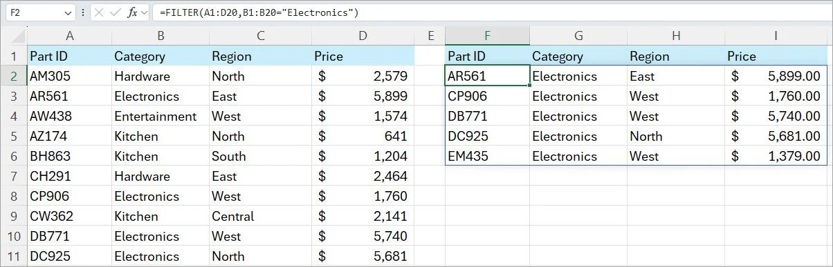
Because this is a dynamic array function, when I enter the formula in cell F2, it automatically fills across multiple cells. This neat little feature is known as spilling. You can see that the results range has a blue outline, and if I click on another cell in the results range, the formula bar is greyed out. This is a visual clue that I’ve entered a spill range.

Now that my data is displayed in the results area, I can edit the formula to show other items. However, it’s a bit clunky to do that, so I’ll make a couple of adjustments to the set up.

First, I’ll move the results down a bit to make some room for a reference area. I’ll add a Category heading, and below that I’ll enter the category I want to filter.

Now I can edit the formula to the following:

=FILTER(A2:D20, B2:B20=G2)

The formula works as before, but now I can adjust the results by typing a different category in cell G2. As a bonus, because this is spill function, I don’t need to worry about using an absolute cell reference ($G$2).

Let’s take it another step.

Currently, if no data matches my criteria, the function returns a #CALC! error. A typical solution to this problem is to nest the formula in an IFERROR function, but in the case of FILTER, we can just use the optional [If empty] argument that’s built right in.

To do this, I’ll adjust the formula as follows to display a more friendly message if no records are found.

=FILTER(A2:D20, B2:B20=G2, “No Match”)

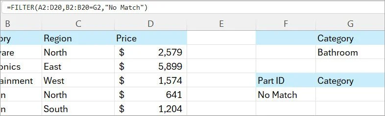
This is looking good, but the function is only based on a single criterion. If I want to find all records where the Category is Electronics, and the Region is Central, I need to modify the formula.

Filtering with Multiple Criteria (AND Logic)

To filter by more than one criterion when using the FILTER function, I need to supply two or more logical expressions for the include argument.

To make this work, I need to use the multiplication * operator. The operator processes my data using AND logic. This means that only records that meet all criteria are returned.

This is because the result of each logical expression is an array of Boolean values, where TRUE equates to 1 and FALSE to 0. Then, the elements of all the arrays in the same positions are multiplied. Since multiplying by zero always returns a zero, only the items where all the criteria are TRUE are processed in the resulting array, therefore only those items are extracted.

In the example, I want to find items where the category is Kitchen, and the Region is South.

In the example, only 2 records are returned, since they meet both of my criteria.

Filter with multiple criteria (OR logic)

Ok, so what if I want to find any item that meets either criterion? To filter data based on a multiple OR condition, you use logical expressions like the previous example, but instead of using multiplication, you use + addition. When the Boolean arrays returned by the expressions are summed, the resulting array will return 0 for entries that don’t meet any criteria (i.e. all the criteria are FALSE), and those entries are filtered out. The entries where at least one criterion is TRUE will be returned.

In this example, simply changing the multiplication to addition in the formula results in 6 results, all of which meet either of my conditions, nice!

Nesting with SORT.

Why stop at filtering when you can sort at the same time?

I want to sort my results in descending order of price. Here’s the way to do it.

=SORT(FILTER(A2:D20,(B2:B20=G2)+(C2:C20=H2),”No Match”),4,-1)

This pulls the chosen category and region then sorts by column 4 (“Price”) from highest to lowest.

Combining FILTER with TRIMRANGE (for the Tidy‑Obsessed)

If your source range might sprout blank rows at the top or bottom, you can wrap it in TRIMRANGE first.

In my small example, the selected range goes from row 2 to row 20, but what happens when the range is larger, (as will almost certainly be the case).

In this example, my formula is only looking at the first 20 rows, but I expect data to be anything up to 100 rows. To allow for this, I’ll edit the formula to include the TRIMRANGE function as follows:

From this =FILTER(A2:D100,B2:B100=G2)

To this =FILTER(TRIMRANGE(A2:D100),TRIMRANGE(B2:B100)=G2)

Adding TRIMRANGE ensures that Excel only checks the real data, not a sea of emptiness. That’s perfect for large workbooks. Check out our article Microsoft Excel using the Trimrange function for more details of how to use this function.

Trim References vs FILTER – A Quick Aside

You might remember from our TRIMRANGE article that popping a dot inside a range (e.g. A1.:.E100) trims blanks without a separate function. Sadly, FILTER doesn’t accept dotted ranges directly (at the time of writing this article!), so stick to TRIMRANGE or Tables when you want auto‑sized inputs.

Bonus Tip

Try converting your source range to an Excel Table (Ctrl + T). Then your formula shrinks to something actually readable.

In my example, I changed the table name to “Inventory”.

=FILTER(Inventory, Inventory[Category]=H1)

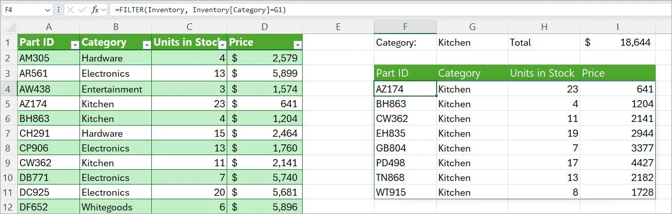
Now there’s no need to worry about row numbers at all. You can just let the Table grow dynamically and let FILTER do its thing.

Check out our article Why you should Convert your Microsoft Excel Lists to Tables for more information.

Things to Keep in Mind

1. FILTER Spills
   Make sure the cells below and to the right of your target range are empty, otherwise Excel complains with “Spill range isn’t blank.”
2. Volatile? Not Exactly, but…
   FILTER recalculates whenever the underlying data or criteria change. On gigantic sheets, pair it with sensible ranges (Tables are perfect).
3. Available in Microsoft 365
   If your colleague’s Excel looks puzzled when you open a workbook full of FILTER formulas, they’re probably on an older version. Time to charm IT into an upgrade. 

Conclusion

The FILTER function brings a fresh level of agility to data analysis in Excel. By letting you define clear, reusable rules in a single formula, it saves time, reduces errors, and keeps worksheets blissfully clutter‑free. Mix it with SORT, TRIMRANGE, or Tables and you’ve got a toolkit that scales from tiny lists to six‑figure datasets without breaking a sweat.

Give FILTER a whirl on your next report and see how quickly those long, sleep‑inducing spreadsheets snap into focus. Then sit back, sip your coffee, and enjoy the moment someone says, “You just saved me hours!”