

Building Computer Skills to Enable Success
Building Computer Skills to Enable Success

Microsoft Excel has introduced yet another new tool. It’s the TRIMRANGE function, and it makes working with dynamic ranges much more efficient. In this article, Mark Finney, Co-Founder and Facilitator at Keystroke Learning, explores the uses of TRIMRANGE.
Barely a day goes by when I don’t use Microsoft Excel for something or other. It’s like a Swiss Army knife for data and calculations, so I love it when a new feature is introduced. I realise that may mean I need to get out more, but I can live with it!
I’ve always been a fan of the TRIM function, which is a simple, but incredibly useful function that punches well above its weight. Now there’s a new function called TRIMRANGE, and along with its little buddy, Trim Refs, I think you’re going to like it. Let’s check them out.
What is the TRIMRANGE Function?
Simply put, the TRIMRANGE function removes empty rows and columns from your specified range. It’s great for creating dynamic ranges that automatically adjust as your data changes. This in turn improves the efficiency of your worksheets and makes them much tidier to boot!
TRIMRANGE syntax
The TRIMRANGE function scans inwards from the edges of a range or array until it finds a non-blank cell, then excludes those blank rows or columns from the range.
=TRIMRANGE(range,[trim_rows],[trim_cols])
|
Argument |
Description |
|
Range |
The range (or array) to be trimmed |
|
trim_rows |
Determines which rows should be trimmed |
|
0 – None 1- Trims leading blank rows 2 – Trims trailing blank rows 3 – Trims both leading and trailing blank rows (default) |
|
|
trim_cols |
Determines which columns should be trimmed |
|
0 – None 1- Trims leading blank columns 2 – Trims trailing blank columns 3 – Trims both leading and trailing blank columns (default) |
How to use TRIMRANGE
Ok, let’s start with a simple example of the TRIMRANGE function before we get into some of the practical ways to use it.
(Note – I would typically use this to extract the data to a different sheet tab, but for the sake of clarity in my example, I’ll keep it on a single sheet).
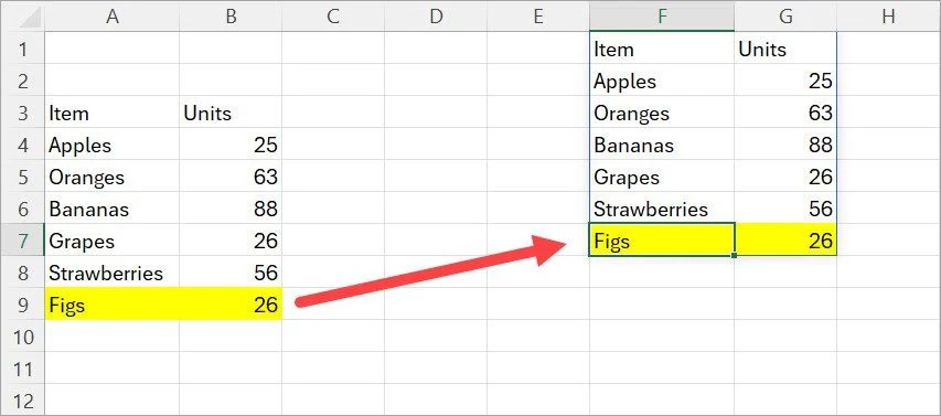
In the spreadsheet below, I want to extract the data from columns A and B to my results area. I’ll use the following steps:
- Click cell F1 (this is my Results area).
- Type =, then select the range A3:B8.
- Press the Enter key.
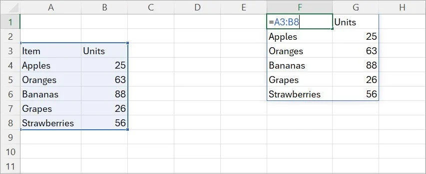
So far, so good. My data is displayed in the Result area. However, what happens when I add some new data to the list? It’s not added to my results, so I’ll need to go back and adjust the formula each time.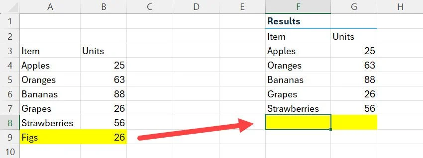
Let’s try it another way.
After deleting the data from the previous example, I’ll use the following steps:
- Click cell F1.
- Type =, then select columns A:B.
- Press the Enter key.
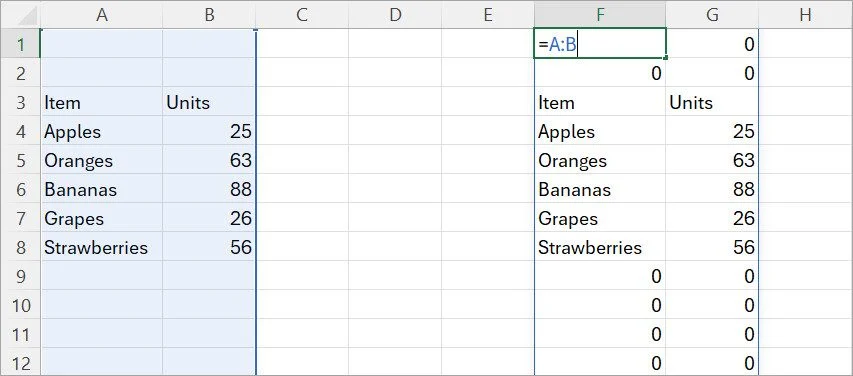
This time, the formula brings the data across, and it includes the empty rows above and below my data. The advantage is that if I add new rows of data, they’ll be included, but it also means that now I have a messy spreadsheet full of zeros. They go all the way down to the bottom of the spreadsheet (over 1 million rows!)
Referencing entire columns in this way is not considered best practice. It’s inefficient because you are basically forcing Excel to check every single cell in the column, even if most of them are empty, and it can slow down calculations.
This is where TRIMRANGE comes in. By automatically removing empty rows and columns from a range, it ensures that Excel only processes cells containing data.
Now let’s use TRIMRANGE.
- Click cell F1.
- Type =TRIMRANGE, then select columns A and B.
- Press the Enter key.
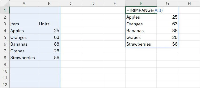
That’s much better! The TRIMRANGE function automatically removed the empty cells above and below my range, leaving me with a clean set of data. If I go back and add or remove rows in my list, it’s automatically reflected in the results area.
With that out of the way, let’s check out a more practical example.
In this instance, I have some sales data, and I need to add the Category field from my lookup table. I’ll use an XLOOKUP function, but I want to allow for more data at the end of the range.
In this formula, I’ll do the following:
- In cell E2, type =XLOOKUP(
- I then select the Lookup Values (that’s currently from D2:D20, but I’ll extended the range to D28 to allow for some new rows of data).
- For the Lookup Array, and Return Array, I used I2:I20, and J2:J20 respectively.
- Pressing Enter; I see the following results.
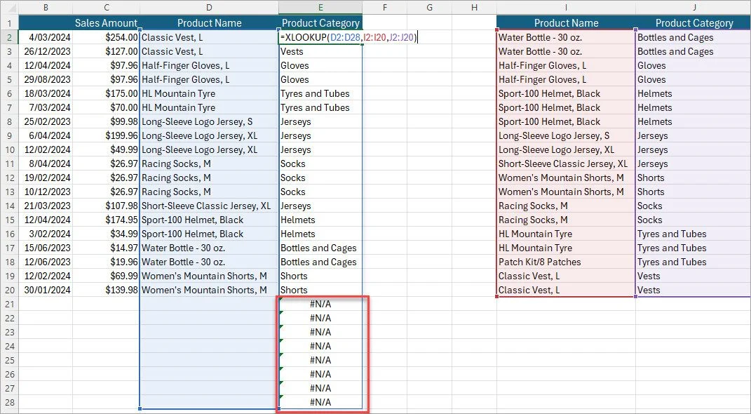
The formula works, but as you can see, I have several rows at the bottom of the range that display the #N/A error message.
At this stage, I could edit the XLOOKUP formula to return a blank instead of an error, but it only hides the issue. The formula is still calculating for the entire range, which means that Excel is doing some extra work. Keep in mind that this is just a small example for the purpose of illustration. In the real world, this spreadsheet would typically be much larger.
Let’s give it a go with the help of TRIMRANGE.
Here’s the new formula in cell E2:
=XLOOKUP(TRIMRANGE(D2:D28),I2:I20,J2;J20)
As you can see in the example below, the TRIMRANGE function removed the extra data at the range, leaving a clean data range behind.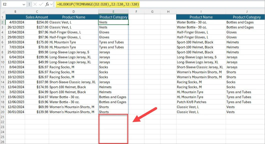
Because the TRIMRANGE function is dynamic, additional rows are automatically included in the results.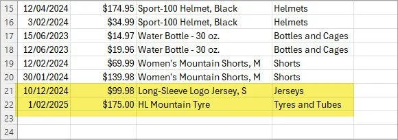
I should mention that in this case I just used the default settings in the TRIMRANGE function, which automatically trims rows and columns. I could have used the options shown in the table at the start of this article to specify that I only needed to trim trailing rows, but since the default settings work just fine, it wasn’t necessary, so I saved myself some extra work.
What about Trim References (Trim Refs)?
It’s all about the dot!
As an alternative to the TRIMRANGE function, we can simply use a dot in our formula. The syntax looks a bit strange at first, but you’ll soon get used to it.
In the table below, you can see that adding one or two dots to the range reference (in this case, A1:E10), behaves in the same way as TRIMRANGE. In other words, using a dot after the colon will remove trailing blanks, and so on.
|
Type |
Example |
Equivalent TRIMRANGE |
Description |
|
Trim All (.:.) |
A1.:.E10 |
TRIMRANGE(A1:E10,3,3) |
Trim leading and trailing blanks |
|
Trim Trailing (:.) |
A1:.E10 |
TRIMRANGE(A1:E10,2,2) |
Trim trailing blanks |
|
Trim Leading (.:) |
A1.:Z10 |
TRIMRANGE(A1:E10,1,1) |
Trim leading blanks |
How to Use Trim Refs
I’ll return to the spreadsheet from by previous examples.
-
Back in cell
E2, I start by deleting the formula.
- Then I enter the following formula:
=XLOOKUP(D2:.D28,I2:I20,J2;J20)
(I made big so you can see the dot after the colon).
- Pressing the Enter key, I now get the same result as I did when using TRIMRANGE, but without the extra function or brackets!
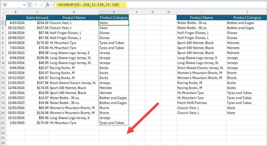
I reckon the Trim Refs dot operator is a nifty way to work with dynamic ranges without the extra work needed to create formulas with the TRIMRANGE function. That being said, if you feel more comfortable using a function instead of those odd little dots, you should go right ahead and use TRIMRANGE.
Some things to keep in Mind
Like any new feature, there are a couple of things worth knowing upfront:
- TRIMRANGE only trims the outer edges
It doesn’t remove blank rows or columns within your data, only the ones at the start and end. So, if you’ve got gaps in the middle, they’ll still be displayed. - It’s a dynamic array function
That means it “spills” its results, so make sure you’ve got some empty cells below and beside the formula to allow for that. - Only available in the latest Excel versions
At the time of writing, TRIMRANGE is part of the Excel 365 lineup and may not be available for you just yet. If your version doesn’t support it, now’s the perfect time to drop some subtle hints to the folks in IT.
Try it yourself
If you’ve got Excel 365 (and the feature has rolled out for you), give TRIMRANGE a spin in one of your existing files. Start with something messy and let it work its magic. You might be surprised how much neater things look with a single formula.
And if you’re still staring at reports with 500 empty rows, well… now you’ve got no excuse!
Conclusion
The addition of the TRIMRANGE function and Trim References operator provides users a significant improvement in Excel’s data management capabilities. By automating the removal of blank cells and improving the accuracy of dynamic calculations, these features enable us to work more efficiently and effectively.
Whether you’re managing complex datasets, consolidating data from multiple sheets, or building streamlined workflows, these tools provide both precision and flexibility to help you with your work in Microsoft Excel.