

Building Computer Skills to Enable Success
Building Computer Skills to Enable Success

Using Linked Data Types in Microsoft Excel
Hi, Excel folks! Do you need your spreadsheet to include company stock prices, exchange rates, or city population details? If so, this introduction to Excel linked data types might just be what you’re looking for.
In this article, Mark Finney, Co-Founder and Facilitator at Keystroke Learning, covers how to set up and use Linked data types in Microsoft Excel, along with some tips to make your spreadsheet even more useful.
About Linked Data Types
Linked Data Types in Excel allow you to turn plain text into rich, connected information drawn directly from online sources.
Linked Data Types are an excellent feature that transform ordinary text into dynamic, data-rich content. Instead of storing just a single value (like “Melbourne”), Excel links that cell to an online data source (powered by Microsoft Bing) and allows you to expand the content to include additional fields such as country, population, or time zone.
When you start using Linked Data Types, each linked cell is a bit like a mini database. It still looks like a normal cell, but it’s holding layers of structured data underneath. You can extract any of that information into other cells, build formulas, or refresh the data whenever you need to. It’s like having a live Wikipedia entry built directly into your spreadsheet.
Why use Linked Data Types?
If, like many of our clients, you’ve ever spent time laboriously copying and pasting geographical or stock data from websites into Excel, you’ll see the benefits of Linked Data Types straight away.
Here are a few benefits:
- Time Saving – no need to keep jumping between Excel and your browser.
- Real Time Data – your data can be updated quickly and efficiently.
- Improve Accuracy – bring live data from the internet.
- Smarter Reporting – add context to your numbers to provide meaning.
Imagine you’re tracking stock information about major companies. Instead of manually typing in each company’s stock price, previous close, and change, you can let Excel fill those details for you. And when something changes, a quick refresh keeps it all up to date.
How to Use Linked Data Types in Excel
Ok, now you have the gist of it, let’s have a look at some examples:
- Stocks – find details of companies, including current stock price, 52 week high, change, and more.
- Currency – these enable quick currency conversions, updated whenever you need.
- Geography – locate information about countries, cities, or regions. Useful for demographics and travel reports.
In this article, I’ll focus on Stocks and Geography. Hey, I don’t want to use up all my mojo in one go, gotta save some for later!
Example – Stocks
The key steps to using Linked Data Types are as follows:
- Type a list of company names (for example, Microsoft, Toyota, Woolworths).
- Select the cells.
- Go to Data > Data Types > Stocks.
- You’ll see small icons appear beside each name, showing Excel has linked them.
- Hover over any cell to view a card full of details such as price, Market Cap, and Headquarters.
In the example below, I’ve opened a Microsoft Excel spreadsheet and entered a list of abbreviations for the companies I want to keep an eye on.

To make this nice and neat, and to provide added convenience, I’ll start by turning the list into a Table by clicking into any cell in the range A1:A11, then pressing Ctrl + T. In the dialog box, I need to tick the box to confirm that my table has headers, then click OK.
The list is converted to a Table, which has several benefits over a typical list. If you want to find out more about Excel Tables, check out my article Why you should Convert your Microsoft Excel Lists to Tables. I’ll wait!

Alright, now for the good stuff!
- First, I’ll select the cells in the Table, then I can go over to the Data tab, where I’ll find the Data Types
- Click on Stocks.
- After a few moments, Excel converts the text to the Stocks data type, and a stocks icon displays to the left of each entry.

Note: If you see a symbol instead of an icon, it means that Excel can’t match the data to an online source. If this is the case, you may need to check for spelling errors, then press Enter to update.
So far, this is looking good. Now I can start to add details.
Back in my spreadsheet example, I’ll widen the first column to give me some room, then I’ll click on the stocks icon to the left of the first entry to see a pop up data card full of details.
In this example, I clicked on ANZ to see the data card.

Adding Further Details
Now that I have the basic information, I’m ready to add some more details. This is where my previous step of turning the data into a Table comes in handy. I don’t need to select the entire list, and the table will automatically expand as I add more information.
In the example below, I clicked on the Add Column icon to the right of the data, then I was able to select an item from the extensive list. In this case, I’ve chosen the industry.

Continuing with the same steps, I can now add more columns as needed. I added Employee numbers and Market Cap.

Example – Geography
For my next example, I’ll use the Linked Data Types to add some geographical information related to the states in my list. (I’ll use a Table again to keep things nice and tidy)
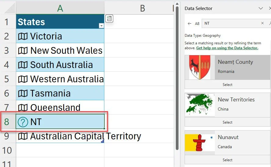
Hmmm… this time I ran into a problem. Excel didn’t recognise NT, so I needed to sort that out. I clicked on the question mark icon to the left of NT, which displayed a list of suggestions on the right. Unfortunately, none of them are correct.
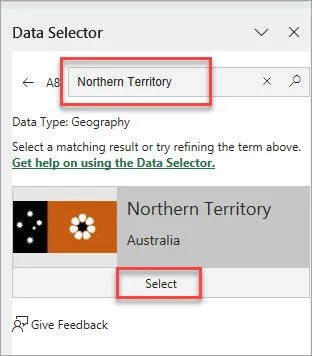
To fix, I typed “Northern Territory in the search box at the top of the Data Selector, then clicked Select at the bottom when Excel found a correct match for my data. Problem solved!
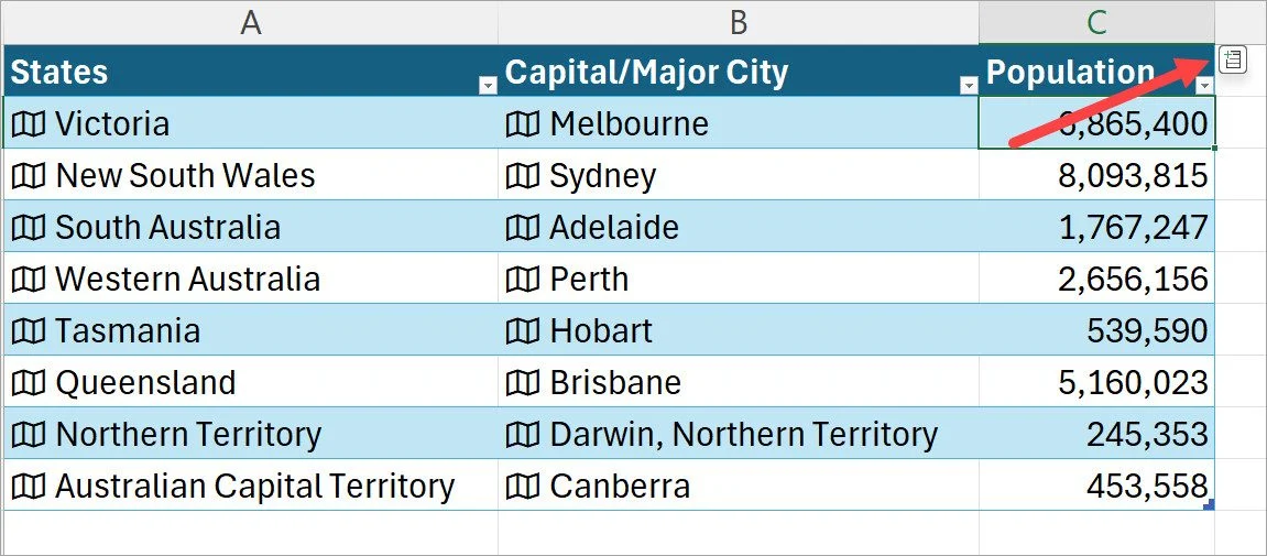
Now my list is set up, it’s time to start adding some content. I’ve added a couple of columns to display the major city and population for each state, but you can add plenty of other details as needed.
Refreshing Linked Data
Because linked data is connected to an external source, it’s easy to refresh it manually or automatically.
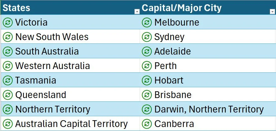
To refresh, just go to the Data tab, then click Refresh All. You’ll see green circles appear beside each item, and few moments later, any details that have changed in the source will be updated in the spreadsheet. Probably more useful when you’re looking at stocks, but you get the idea!
- To view or modify a connection, select the cell and open its Data Type Card.
- If a cell displays a #FIELD! error, it may mean the link is broken or the source is unavailable.
Troubleshooting and Limitations
If you find your data isn’t refreshing, or is incorrect, you can try the following:
- Check your internet connection.
- Make sure the text matches a recognised entity.
- Try reconverting the data type from the ribbon.
While Linked Data Types in Excel are incredibly useful, they’re not perfect. Here are some things to keep in mind:
- Not every term is recognised (especially brand names or smaller companies).
- Some data types are only available with a Microsoft 365 subscription.
- Data accuracy depends on the provider.
- Limited functionality when working offline.
You should treat them as a time-saving assistant, not a substitute for critical research.
Extra Tips
- Rename fields – If the inserted data header isn’t clear, just edit it. Don’t worry, it won’t break the link.
- Use Tables – Converting your range to a Table (Ctrl + T) makes updating and sorting easier.
- Add visuals – Conditional formatting and sparklines make live data more meaningful.
- Explore the Card View – Click the Data icon in a linked cell to see all available data at a glance.
Conclusion
Linked Data Types in Excel can transform the way you work with information. They save you time, improve accuracy, and make your spreadsheets far more engaging, all while staying connected to real-world data.
If you’re ready to try it, start small. Pick one dataset (maybe a list of cities, clients, or companies) and try converting it. Explore the data cards, extract a few fields, and see how dynamic your sheet becomes.
Excel has come a long way from being “just a calculator.” With linked data types, it’s now your research assistant too, ready to fetch the facts while you focus on the bigger picture.